3D Scene Reconstruction with NeRF

3D scene reconstruction and novel view rendering with NeRF (Neural Radiance Fields)

December 2024

Abstract

This project implements a NeRF-based framework that represents a 3D scene in a compact way and render novel views given a number of 2D views of the same static scene. It integrates positional encoding, stratified sampling, and volumetric rendering.

Introduction

Neural Radiance Fields (NeRF) are powerful tools for 3D scene reconstruction. This project focuses on employing NeRF to represent scenes as mappings of 3D positions and viewing directions to RGB color and density. By leveraging positional encoding and efficient rendering techniques, this implementation enhances the quality and realism of synthesized scenes.

Core Components

Below are the key components of the NeRF framework.

Figure 1: Core procedure of the neural radiance field scene representation and differentiable rendering procedure [1]

Positional Encoding

The positional_encoding function applies sinusoidal transformations to map continuous coordinates into higher-dimensional space, enhancing the ability to model high-frequency variations in scenes.

\gamma(x) = [\sin(2^0\pi x), \cos(2^0\pi x), \dots, \sin(2^{L-1}\pi x), \cos(2^{L-1}\pi x)]

Ray Sampling

Rays are sampled using get_rays and stratified into points along the ray using stratified_sampling. This ensures uniform coverage of the 3D scene, crucial for accurate density and color estimations.

t_i = t_{near} + \frac{i-1}{N} (t_{far} - t_{near}), \quad i = 1, \dots, N

NeRF Model Architecture

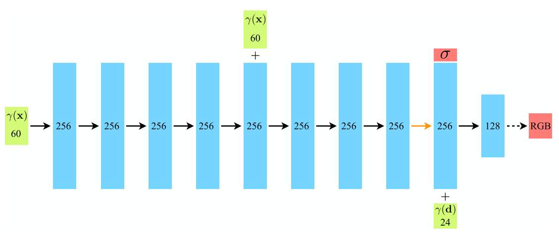
The nerf_model class defines a neural network architecture with:

10 fully connected layers with ReLU activations.
A skip connection at the fifth layer to propagate input features.
Separate branches for density prediction and feature-vector computation for color.

Figure 2: NeRF architecture for 3D scene reconstruction [2]

Volumetric Rendering

Colors of rays (pixels) are computed using the volumetric rendering equation. The method aggregates densities and RGB values along each ray to synthesize a 2D projection of the 3D scene.

C(r) = \int_{t_{near}}^{t_{far}} T(t) \sigma(r(t)) c(r(t), d) \, dt

T(t) = \exp\left(-\int_{t_{near}}^t \sigma(r(s)) \, ds\right)

From the above formulas, we have the following discrete approximations:

\hat{C}(r) = \sum_{i=1}^N T_i (1 - \exp(-\sigma_i \delta_i)) c_i

T_i = \prod_{j=1}^{i-1} \exp(-\sigma_j \delta_j), \quad \delta_i = t_{i+1} - t_i

Results

Figure 3: Volumetric rendering result from the implementation, with σ = 0.2

Figure 4: The novel view the project try to render, before training

Figure 5: The novel view the project try to render during the training process

Figure 6: The novel view the project try to render, after training

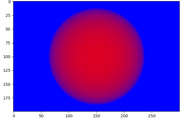
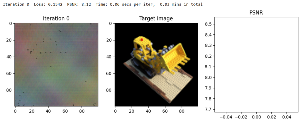
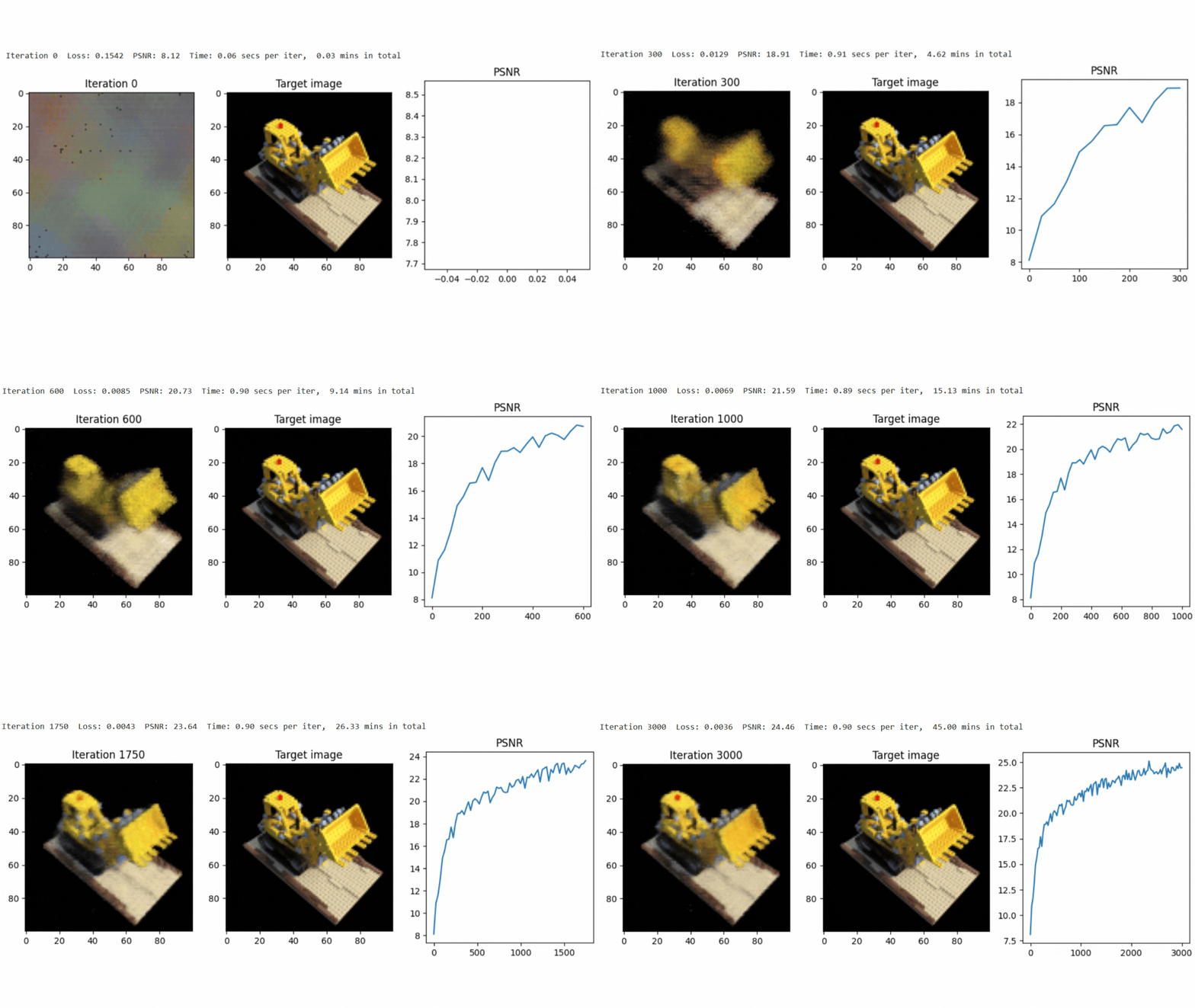
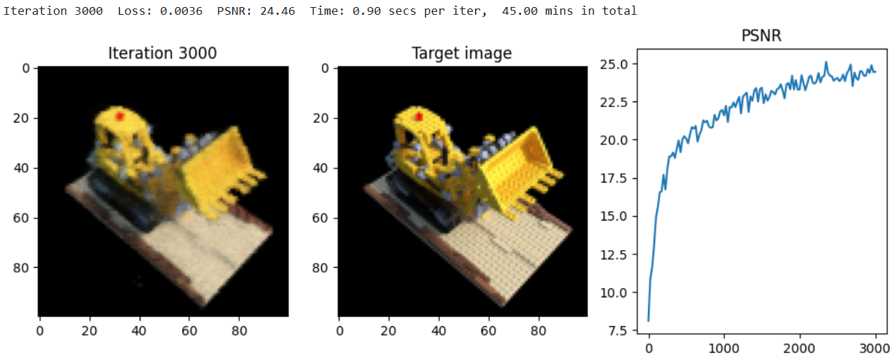
The implementation achieved a PSNR of around 25.0 after 3000 iterations, demonstrating the effectiveness of NeRF in scene reconstruction.

\text{PSNR} = 10 \cdot \log_{10} \left(\frac{R^2}{\text{MSE}}\right)

Here, $R$ represents the maximum pixel intensity, and $\text{MSE}$ is the mean squared error between the reconstructed and ground truth images.

Conclusion

This project successfully showcases the NeRF framework's potential for 3D scene reconstruction. The combination of positional encoding, ray sampling, and volumetric rendering allows for high-quality scene synthesis.

References

[1] Mildenhall et al. (2020). NeRF: Representing Scenes as Neural Radiance Fields for View Synthesis. In arXiv preprint arXiv:2003.08934.
[2] Towards Data Science. (2020). NeRF: Representing Scenes as Neural Radiance Fields for View Synthesis.

Anh-Quan Pham